An Introduction to Neural Networks

At Koi, neural networks play a big part in our trading models. This article aims to provide a basic understanding of how neural networks work, and are used in decision making.

What are Neural Networks?

Figure 1: Structure of a Neural Network

The term “Neural Network” was inspired by the way biological neurons signal to one another within the brain. Neural networks are typically composed of artificial neurons called “nodes” which are connected to each other by “edges”. Each node is arranged into a certain layer within the network.  

The three main classifications of node layers include: an input layer, hidden layers and an output layer. The goal of a neural network is to generate a prediction or classification at the output layer, based upon data from the input layer. 

How does a Neural Network Work?

Neural networks work by passing information from layer to layer along connecting edges. As information is passed to each layer, the nodes that make up the layer process this information, derive insights, and then pass them on to the next layer. To simplify this process, let’s use an example. 

Assume that Sarah has a list of stocks and has asked for your help to decide which ones to buy. Her three main stock evaluation criteria include that the company pays a dividend, has an environmental, social, and governance (ESG) rating above AA, and has sales growth of over 15%. 

Figure 2: Sarah’s Stock Criteria

To help Sarah select which stocks to buy, you decide to create a neural network composed of an input layer and an output layer. The input layer will be made of three nodes representing each one of Sarah’s criteria. Each input node will be connected to the output layer by a weighted edge. The weight of each edge will represent the importance of the input neuron to the output layer. The output layer will yield either a 0 (don’t buy) or a 1 (buy), determined by whether the weighted sum of the inputs is greater than some threshold value.  This neural network is illustrated in figure 3.  

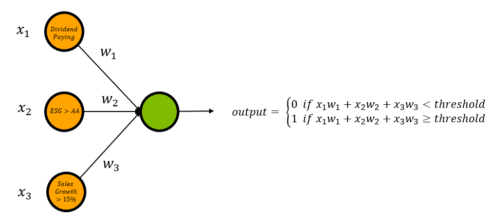
Figure 3: Sarah’s Stock Selection Neural Network

In order to represent the three node criteria, we will assign each node a binary variable (x1, x2 and x3). For instance, we’d say x1 = 1 if the stock is dividend paying, and x1 = 0 if the stock is not. Similarly x2 = 1 if the stock’s ESG rating is higher than AA, and x1 = 0 if it is not. Again this is repeated for x3 and sales growth.

Now, assume that Sarah is very environmentally conscious, so much so that she will not buy a stock with an ESG rating lower than AA. To ensure this is factored into the decision making process you assign edge 2 a value of 5 (w2=5). Sarah also cares that the stock has a sales growth of over 15%, but this is second to the ESG rating. You assign edge 3 a value of 4 (w3 = 4). Finally, Sarah would prefer if the stock was dividend paying, but does not mind if this criteria is not met as long as the other two are. Correspondingly, you assign edge 1 a weight of 3 (w1=3). Notice that the weights of each edge correspond to the importance of the input neuron to the output. Our updated weights are as follows.

Figure 4: Neural Network with Updated Weights

Testing the Neural Network

Continuing with our example, suppose you choose a threshold value of 8 for the output neuron. This means that in order to output a 1 (buy), the weighted sum of the input layers must be greater than or equal to 8. 

Figure 5: Choose threshold parameter to be 8

To test our neural network, Sarah gives us two lists of stocks. The first list includes three stocks that Sarah has classified as either “buy” or “sell.” We call this list of data our “training data.” Training data is data where both the inputs and outputs are labeled with the correct classification. Our algorithm “learns” from these data sets by adjusting parameters, for example the weights of the edges, so the input produces the correct output. The training data is shown in Figure 6.

Figure 6: Training Data

The second list includes three stocks that are not classified. We call this type of data “unlabeled data,” meaning that for every input there is no corresponding output classification. Instead, it is the algorithm's job to determine the correct classification. For this example we will label this data our testing data, as shown in figure 7.

Figure 7: Testing Data

To test our parameters, we will input the training data (stock A, B and C)  into our neural network, and see if we get the same results as the data output labels (Buy, Buy, Don’t Buy). Our results are shown in Figure 8.

Figure 8: Training Data vs Neural Network Result

As seen in figure 8, after running each input through the neural network we find that all three stocks were classified with their correct labels. Because of this success we will not change any of our test parameters (we keep our weights the same), and move on to classifying our unlabeled “testing data.” Our testing data is classified in Figure 9.

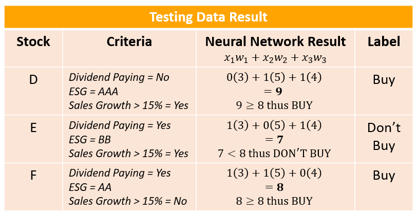
Figure 9: Classified Testing Data

Conclusion

In conclusion, this is a simplified example of a neural network that illustrates how a single output node can weigh up different kinds of evidence in order to make decisions. By adding more node layers and varying the weights and thresholds of these layers, we can see how a complex neural network can make very sophisticated decisions and determine data correlations otherwise impossible for a human to discern.